How To Draw A Stock Control Graph Using Matplotlib

Using Matplotlib To Analyze Stock Trends

In this tutorial, nosotros'll learn how to leverage data visualization in Python to examine trends in companies' valuation, liquidity, and operational effectiveness.

Nosotros'll also exist pulling in historical financial information from my API on TenQuant.io. You lot can register an API key for free on the site — you'll get admission to financial statements and pricing dating as far back as 2010, sourced directly from the SEC's database. Annals your API key and and go along information technology somewhere rubber.

Before starting whatever major project, information technology's best to plan it out. Allow's write out some class and method stubs, and import some libraries we're going to utilise. Open your Python IDE or editor and write the following code:

          import matplotlib.pyplot equally plt; plt.rcdefaults()
import numpy as np
import matplotlib.pyplot as plt            
import requests
                    class StockPlot:
            def __init__(self, ticker):
            self.ticker = ticker                      # plots a graph of our information over time
            def plot(self):
            pass                      # returns a Dictionary of bespeak-in-fourth dimension financial information
            def get_financials(self, date='20200101'):
            pass                      # runs calculations and returns the electric current ratio: current avails - electric current liabilities
            def get_current_ratio(self, financials):
            pass                      # returns enterprise value to sales
            def get_ev_to_sales(self, financials):
            pass                      # returns ev to ebit, excluding unusual items
            def get_ev_to_ebit(self, financials):
            pass

This is a loosely object-oriented approach — notice that nosotros're breaking downward diverse specific calculations into single methods. This helps the states maintain cleaner code and add new features in easily.

Let's start past pulling downwardly financial information from TenQuant.io:

          def get_financials(cocky, date='20200101'):
            API_KEY = 'YOUR_KEY_HERE'                      # utilise an f-string to build your query
            query_url = f'https://api.tenquant.io/historical?key={API_KEY}&date={date}&ticker={self.ticker}'
            financials = requests.get(query_url).json()
            return financials

This method will render a JSON representation of cleaned, standardized financials at a specified engagement.

Next, we need to run some basic calculations on this financial data then we can visualize trends. I picked the electric current ratio (since information technology allows united states to see if a firm tin can afford to run across its obligations on time) EV-to-sales (a valuation metric, measuring the cost of acquiring a visitor confronting the revenues it generates), and EV-to-EBIT, which is another valuation metric often used to model how expensive a visitor would be to acquire.

Let's start with the electric current ratio:

          def get_current_ratio(self, financials):
            current_assets = financials['currentassets']
            current_liabilities = financials['currentliabilities']
            return current_assets / current_liabilities

Equally you lot tin see, this is a adequately unproblematic calculation. A current ratio beneath 1 or 1.5 may betoken that a firm is in danger of beingness unable to meet its obligations in the next year unless it generates plenty new cash flow to pay them downward.

Next up is EV-to-sales. Enterprise value is defined as: [Market Cap] + [Debt]- [Cash and Equivalents]. Because some financial reports are non for a full year, we'll also need to annualize the revenues reported.

          def get_ev_to_sales(cocky, financials):
            sales = financials['revenues']
            elapsing = financials['elapsing']  # figures are from this many quarters
            greenbacks = financials['currentassets']  # substitute current assets for greenbacks
            debt = financials['liabilities']
            market_cap = financials['marketcap']                  annualized_sales = sales / (duration / 4)  # annualize sales
                              ev = market_cap + debt - cash
              ev_to_sales = ev / annualized_sales
                              return ev_to_sales

Lastly, nosotros'll calculate EV-to-EBIT. Depending on how it is calculated, EBIT (earnings before interest and taxes) can exist calculated from either the lesser upwards (take net income, add back interest and taxes) or the summit downwards (just operating income). Nosotros'll take the old approach, since information technology is a little more than in the spirit of the metric, but may include non-operating income and expenses.

          def get_ev_to_ebit(self, financials):
            net_income = financials['netincomeavailabletocommonstockholdersbasic']
            interest = financials['interestanddebtexpense']
            taxes = financials['incometaxexpensebenefit']
            ebit = net_income + involvement + taxes*(-1)  # taxes are recorded as an absolute effigy: income/(loss)                      duration = financials['duration']  # figures are from this many quarters
            greenbacks = financials['currentassets']  # substitute current assets for cash
            debt = financials['liabilities']
            market_cap = financials['marketcap']                      annualized_sales = ebit / (duration / 4)                      ev = market_cap + debt - cash
            ev_to_ebit = ev / annualized_sales                      return ev_to_ebit

Great! Now, nosotros need to visualize these data points using Matplotlib, a powerful Python information visualization tool. Pull in your data and fix it for plotting:

          def plot(cocky):
            dates = ['20160101', '20170101', '20180101', '20190101', '20200101']
            x_pos = np.arange(len(dates))                      # let'south use some fancy list comprehension
            # it's fun and makes for cleaner code.
            financials = [self.get_financials(d) for d in dates]
            current_ratios = [self.get_current_ratio(f) for f in financials]
            ev_to_saless = [self.get_ev_to_sales(f) for f in financials]
            ev_to_ebits = [self.get_ev_to_ebit(f) for f in financials]

Now, nosotros just need to generate a few plots using Matplotlib.

          # window 1
plt.figure(1)
plt.bar(x_pos, current_ratios, marshal='center', alpha=0.v)
plt.xticks(x_pos, dates)          plt.ylabel('Current Ratio')
plt.xlabel('Date')          # window 2
plt.figure(2)
plt.bar(x_pos, ev_to_saless, align='center', alpha=0.five)
plt.xticks(x_pos, dates)          plt.ylabel('EV/Sales')
plt.xlabel('Date')          # window 3
plt.figure(3)
plt.bar(x_pos, ev_to_ebits, align='centre', blastoff=0.five)
plt.xticks(x_pos, dates)          plt.ylabel('EV/EBIT')
plt.xlabel('Date')          # plot graphs
plt.show()

Finally, add in this code and requite your program a run!

          if __name__ == '__main__':
            sp = StockPlot('AAPL')
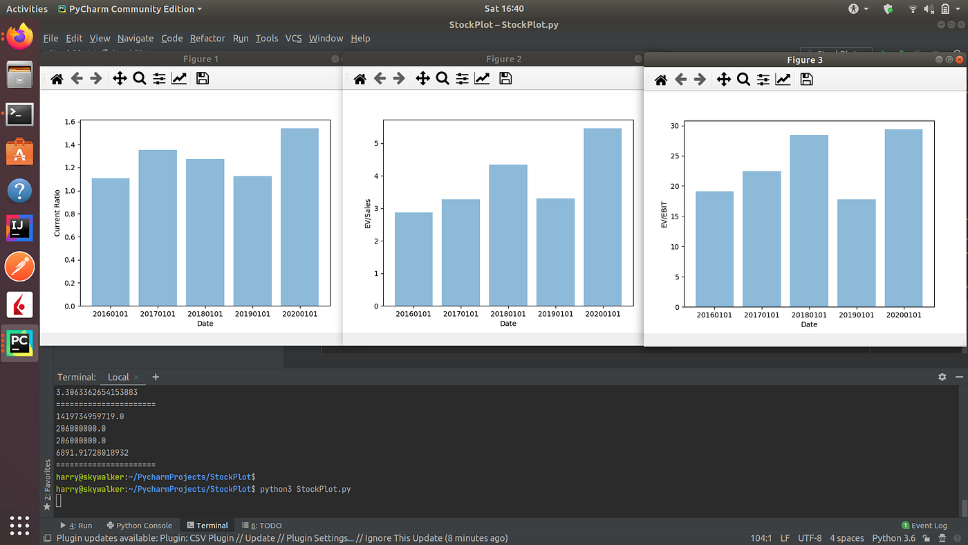
            sp.plot()

You should see iii cute graphs documenting Apple's trends over time.

As e'er, play around with this code and get in your ain. Try plotting new variables, improving the logic, or trying out new chart types. Happy Python-ing!

Cheque out the total project on my Github: https://github.com/hsauers5/StockPlot